
Tangram-II is a suite of tools for the modeling, analysis, and evaluation of computer and communication systems. It features among other things, a modeling environment in which the user can provide a high-level description of a system and later on, obtain performance measures from it. If the system being modeled satisfies the necessary conditions to be represented as a Markov chain, Tangram-II can generate its infinitesimal generator automatically and calculate its state probabilities, for either transient or steady state behavior.
In this tutorial you will perform the basic steps in the Tangram-II modeling environment through a simple model of a queueing system that employs a push-out policy for rejecting customers. After reading this tutorial, you should be able to:
In all further discussions, I assume that you have already downloaded and installed Tangram-II, and that you can work your way around the user interface. You can download the tool at http://www.land.ufrj.br/tools/tangram2/tangram2.html. There you will also find installation instructions.
This tutorial was written and executed with the 2.0 version of Tangram-II, but you should be able to run it on any version newer than this, since the tool is designed with backwards compatibility in mind.
Consider the following queueing system, that could represent an output link at an network router. It receives two kinds of customers: regular ones (which we will tag as red for ease of display), and others marked as having higher priority of service (which we will tag accordingly as blue). This priority scheme determines the scheduling policy at the server. A red (regular, low priority) customer will only be selected for service if there are no blue (high priority) customers currently available at the waiting queue. The scheduling policy is strictly non-preemptive: a customer being served will not be removed from the system until it finishes its service time, in any situation.
The system can store up to N customers including the one at service. There is no kind of reservation for customers of a given class, i.e., the upper limit N is set over the total number of customers, without regard to each type. Red customers arrive according to a Poisson process with rate Rr, and blue customers as another Poisson process with rate Rb instead. Service times for both kinds of customers are exponential with mean X.
In case a red customer arrives to find the system full, i.e., with N customers, it is rejected (lost) instantly. A blue customer that happens to arrive at such conditions, will have the opportunity to push a red customer out of the system, if one such customer is at the waiting queue (but not in service, since the discipline is non-preemptive). Given these condition are met, the push-out event happens with a probability p.
Now let us focus on a Tangram-II model that represents the system previously described. In Tangram, the system is described as a collection of components called objects. An object may be described in terms of its properties and its behavior. In this exercise, we will only be concerned with understanding an object's properties, and delay the discussion of behaviors to another tutorial.
First of all, you will need to download the model we will be using throughout this tutorial.
Now, run Tangram (this should be as easy as typing 'tangram2' from your favorite command line shell) and go to the Modeling Environment. There, open the model file you downloaded and go to the model specification in TGIF. The picture below illustrates the sequence of windows you should see in doing this.

Once you have TGIF on your screen, you should have a general view of the model, as in the picture below.
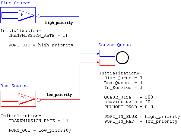
If you take a look at the model, you will see it is composed of
three objects, each one with an unique name. Two of them, Blue_Source
and Red_Source,
represent the Poisson processes of blue and red customers,
respectively. The third object, Server_Queue,
stands for the actual server along with its waiting queue. In the
picture, I have set the sources with different colors, but this has only
illustrative purposes, i.e., the sources behaviors are in no way at all
affected by its color on the display.
You may have also noticed that both sources seem to be "connected"
to the server object. That is indeed correct, even though the two lines
named low_priority
and high_priority
only have the purpose of illustrating this connection. What makes the
real connection is just a little less visual. Notice that each source
has a "port" embedded into it,
which are named PORT_OUT
in both sources. The server, on the other hand, has two more ports,
named PORT_IN_BLUE,
and PORT_IN_RED.
These ports are some of the properties that an object may have, as I
have mentioned before.
You can probably see that the port in Blue_Source is assigned to the same value as PORT_IN_BLUE at Server_Queue (the string high_priority, which in Tangram-II we refer to as a "wire"). This is what connects Blue_Source to Server_Queue. Similarly, the red source is connected to the server through a wire named low_priority. These connections enable the sources to tell the server each time a customer is generated.
By now, you have already noticed the Initialization
text below each object. In order to explain that, let me first tell you
about an object's attributes. In TGIF, objects have what we call
attributes. In order to see Blue_Source's
attributes, right-click the object and then open the menu Edit Attribute in
Editor. There, you will probably find six attributes as in the
picture below.
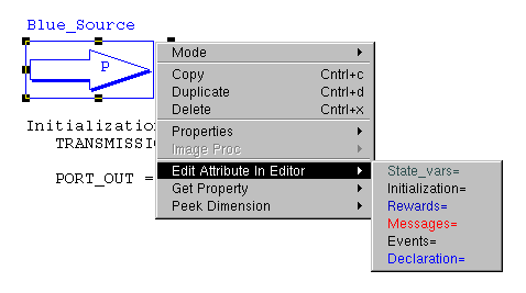
For this tutorial we will only be interested in two of them: Declaration and Initialization. In the Declaration part, you will find the model's properties as they were declared. For both sources, the Declaration part should contain the following:
| Const Float: TRANSMISSION_RATE; Port: PORT_OUT; |
Here, Const is just a keyword to specify that the following declarations will be of constants. In Tangram-II (as in any other reasonable language), constants are assigned one value once, and remain with this value during their entire lifetime. As you can see, there are two constants declared in the source object. The first one, is a floating-point real valued constant named TRANSMISSION_RATE, which specifies the rate of the Poisson process that the source represents. Taking the two sources, these constants are equivalent to the parameters Rb and Rr in the original system specification. The other constant, as we have already seen, is the port that enables the source to send its customers to the server object.
Speaking about the server object, if you take a look at its Declaration attribute, you should see:
| Var Integer: Blue_Queue, Red_Queue, In_Service; Const Integer: QUEUE_SIZE; Float: SERVICE_RATE, PUSHOUT_PROB; Port: PORT_IN_BLUE, PORT_IN_RED; |
Now you can see that besides constants, this one object has properties declared under the keyword Var. This just means that these are variables that define the state of your object. They are initialized to some value as a starting state, and the object's behavior is free to change this value during time. The server object has three state variables:
If you take the entire collection of state variables from all the
objects in the model, then you have a tuple that can be seen as the global system state. Since the
sources do not have state variables, the system state for this model
should be the tuple:
Where X.Y is just the standard notation to say that object X has a property named Y. If the system satisfies the conditions to be considered a Markov process (which is the case in this model), this will be the state of the chain that will be generated.
Finally, notice that the server object also has some extra constants declared. First, there is the integer valued QUEUE_SIZE, which defines the maximum number of customers in the server and waiting for service (just like the parameter N in the system specification). The SERVICE_RATE constant is the rate parameter for the exponential distribution of service times, which is equivalent to X -1 in the original system. Last, but not least, PUSHOUT_PROB is the probability p that a blue customer will push-out a red customer if the required conditions do happen.
Now we can finally focus on the really important stuff. Each object
also has an Initialization
attribute, which is the place where you are supposed to initialize the
numerical values to constants and state variables in the model. We have
already seen that ports are assigned to wires, in order to connect
objects, but now I want you to focus on the other properties we have
just mentioned.
The TRANSMISSION_RATE
in Red_Source
is set to 10 customers per time unit, while in Blue_Source
it is set to 11 (just a little higher). We also set the QUEUE_SIZE
to 100 customers and SERVICE_RATE to
20. The PUSHOUT_PROB
is initially set to 0, which is equivalent to considering a system that
does not employ push-out. The example is set like this intentionally, so
you can first see what the system behaves like without the push-out
discipline. Later on, we will change these parameters and see what
happens.
Once you feel you have understood the basics of the model description, it is time to generate the Markov chain associated with this model. This step is pretty easy, once the model is correctly specified. Assuming you have not changed the model you downloaded, then there will not be any problems here. Simply click the button for mathematical model generation, in the modeling environment's main window, and press the button labeled Extract, as indicated in the picture below.

The model's state variables will show up in the table, and all you
have to do is fill in the maximum values for each one of them.
Since Blue_Queue
and Red_Queue
represent the respective amounts of blue and red customers in the
system, these variables have a maximum equal to the QUEUE_SIZE
constant defined in the server object. That one had a value of 100, so
this should be the number to type in the table. On the other hand,
we defined In_Service
as being in the set { 0, 1, 2 }, which gives us the maximum value of 2
for this variable. Do not worry about the other parameters in this
window as they will not be of any use for us in this example.
Now hit the Generate button and take a look the command line terminal where you called 'tangram2' at first place. The Markov model is being generated and if everything is correct, it should end up having a total of 10101 states. If you get any sort of error message, make sure you have not messed up the model and typed in the correct maximum values. If you are unsure about having changed the model, just download it again.
After having generated the Markov chain, you can finally solve its balance equations for steady state probabilities. Going back to the modeling environment's main window, open the analytical model solution window, as shown below.

Make sure you select the Stationary and Exact tabs, and GTH no block as the solution method. Then press the Evaluate button and wait until the the solution method finishes its job.
Finally we can get to the point of taking our model's performance measures. Nevertheless, to keep things simple, we will focus on three quantities:

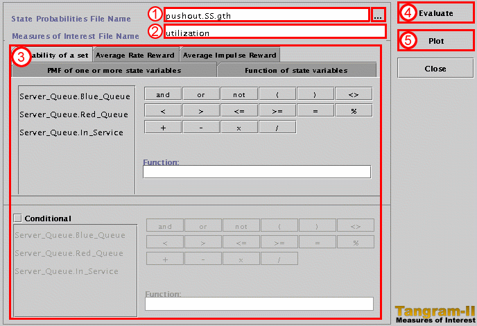
Let us see how we define our three measures of interest with the
Tangram-II panels from step 3.
The system utilization can be defined as the probability the server
is busy. For this we can select the Probability
of a set tab. Click the variable Server_Queue.In_Service
at the list on the left. Notice that the interface automatically puts
the variable at the text field labeled Function
on the right to the list. Now press the button <>
which stands for the operator "is different from". Then, complete the
text field to form the expression:
Now, let us stop for a moment and think about what we just did.
The Probability
of a set tab, lets you specify a boolean expression with your
state variables, and it calculates the probability that expression is
true in your model. Now, if you are asking how does Tangram-II do that,
the answer is simple. All it has to do is open the steady state solution
file and sum the probabilities of all states where your expression is
valid. So, in the end, when you specify the expression Server_Queue.In_Service
<> 0, it simply sums the probabilities of states where the
variable Server_Queue.In_Service
is different from 0, i.e., where it is either 1 or 2. In fact, we could
also have used the expression:
To see the result, open Plot window and select the utilization measure from the list as shown below.
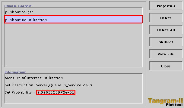
We now have the result for our measure of interest. Before heading for our next one, let us try to calculate the utilization once again, by using a different definition.
Another way to obtain the system utilization by considering an indicator random variable that has value 1 in states where Server_Queue.In_Service is different from zero and 0 otherwise. We can do this by selecting the Function of state variable tab and inputing the same expression as before:
Evaluating the utilization with this definitions yields the same result. But now, we have the utilization is defined as the expected value of the indicator variable we just mentioned. Selecting this measure at the plot window will show what we expected; that the measures indeed are the same. Although this redundancy of definitions may seem silly, it will prove itself useful for obtaining our next measure.
In order to calculate the throughput for the red customers, we can define it as the expected value of a random variable defined as the SERVICE_RATE when a red customer is at service and zero otherwise. In order to obtain that measure, we can use the Function of state variable tab, typing the expression:
In the same reasoning, we can get the throughput for blue customers with the expression:
As an extra feature, notice that we can obtain the rate at which customers of a certain class are lost by subtracting its arrival rate (the parameter in the source object) by the throughput of the same class. This make sense intuitively, since if X customers per time unit arrive at the system and only Y (Y < X) leave the system, it means that X-Y could not get inside. Evaluate the loss rates for each type of customer as a quick exercise.
As our final measure, let us evaluate the expected response for each class of customer. We could define complicated expressions for this, but it turns out that using a little bit of thinking leads us to an easier result. Let us first calculate the mean number of customers of each kind in the system. We can do that by selecting the PMF of one or more state variables tab and adding the state variable corresponding to the class of customers we want to measure. Evaluate the measure for both customers and open up the plot window. Press the Properties button and change Data Style to impulses. Select both measures in the list and click the GNUPlot button. you should see the following graphic:
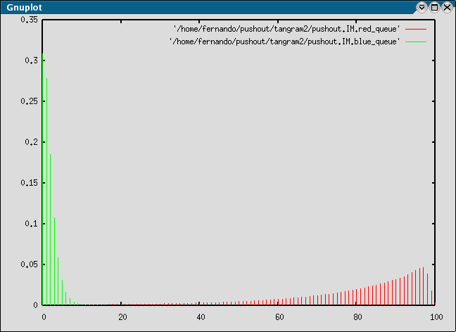
You also know the expected value for each of these distributions by
selecting them at the plot window list and looking the text that shows
up below it. Finally, if you remember Little's result, you can get the
expected response time by dividing the expected number of customers
divided by the throughput of customers. So, dividing the expected number
of red customers by the throughput of the same kind we have the response
time for these customers. Of course, the same applies to blue customers
as well.
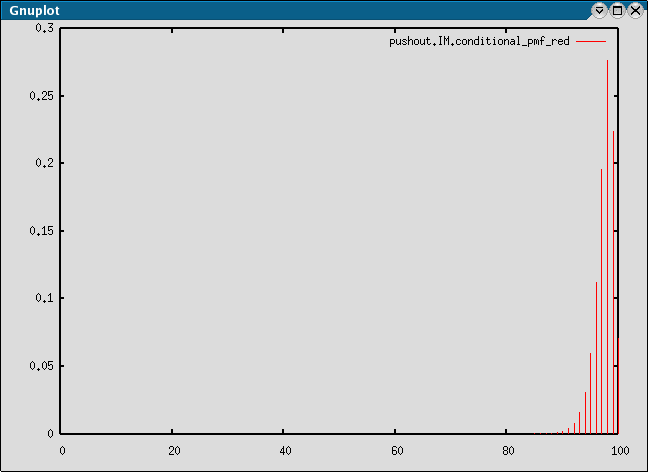
Another related measure we could get is the following: consider a
customer who arrives and finds the system completely full. What is the
distribution of the number of red customers in the system, in this
particular situation? Remembering the PASTA property, we have that this
is conditional PMF of the variable Server_Queue.Red_Queue,
given that the system is full. Tangram-II can easily calculate that, if
you can specify the condition correctly. First, select the PMF
of one or more state variables tab and add only the Server_Queue.Red_Queue
variable to the list to the right. Now check the Conditional
box and type the following expression in the Function
text field:
This will calculate the PMF defined by:
Which, for this example, should look like the following, once plotted:
Now let us do the really important job, understand how the system performance behaves. In this session, I will assume that you have understood the whole process of generating the Markov chain, solving, and taking measures from it. I may introduce some new concepts but I will try not to repeat things from the previous sections.
You can see, summarized in the table below, the results that I got for the measures discussed (rounded to 5 decimal places), and if you did everything correctly, you should have the same values.
| Measure |
Red |
Blue |
| Throughput |
9.52034 |
10.47237 |
| Loss Rate |
0.47966 | 0.52763 |
| Expected
Response Time |
8.31460 |
0.79396 |
| System |
||
| Utilization |
0.99964 | |
What I want you to pay attention is that the fact the loss rate of blue customers is greater than that of red customers. Please remember that although the loss rates in this example are between 0 and 1, they are NOT probabilities, but actual rates instead. A loss rate of 0.5 for blue customers means that during a unit time, 11 customers arrive on average (the Poisson process parameter), but 0.5 (on average) do not enter the system because it is full. To get loss fractions you should divide the loss rates by the correspondent input rate.
Anyhow, blue customers suffering higher loss rates than red ones is very bad since blue customers are the ones who are supposed to receive high priority. What happens is that the system is saturated, i.e., its total input rate (10+11=21), is greater than its capacity (20). In these case, the utilization will be very high (close to 1) and losses are expected to happen somewhat more frequently as indicated by the loss rates. Since there is no push-out (we have made PUSHOUT_PROB equal to 0), the class of customers who is going to be more penalized by the system's state of saturation is going to be the one with higher arrival rate.
We need a way of making sure that the priority scheme is taken into account even in these situations. That is why we may want to implement a push-out discard discipline instead of the usual droptail. Now you will change some parameters in the initial model and repeat the whole process of generating, solving, and taking measures from the Markov chain.
First of all, go back to the model description in TGIF. Edit the Initialization attribute from the Server_Queue object and change the PUSHOUT_PROB to 0.9. This means that if a blue customer arrives to find the system full, having at least one red customer not in service, it has 90% probability of being able to push it out and enter the system. Now it is time to do it all over again. Generate the chain, solve it using GTH no block, and get the measures of interest.
You should notice that the utilization does not change, since the push-out merely changes one customer for another, i.e., it does not improve the general performance of the system. The real differences are in the per-class measures, as you can see below.
| Measure |
Red |
Blue |
| Throughput |
9.04547 | 10.94724 |
| Loss Rate |
0.95453 |
0.05276 |
| Expected
Response Time |
8.73280 |
0.15935 |
| System |
||
| Utilization |
0.99964 | |
Now that you have done the whole thing twice, you will do it twice more :-). Repeat the two previous runs (with PUSHOUT_PROB equal to 0 and 0.9), but with the SERVICE_RATE constant doubled to 40. Compare both results to the ones you have already obtained for the system with capacity equal to 20. Explain what happens and most importantly, why it happens. This one, I will leave to you as an exercise, so enjoy your time!
We have seen how to generate a Markov chain from a Tangram-II model, solve its balance equations for the steady state probabilities, and take interest measures from it. All of this, with a practical application to the performance evaluation of a simple priority queueing system. There is still a lot more you can do with Tangram, like creating your own objects, solving for transient state analysis, and simulating, but these things will have to wait for a another tutorial.